Probability density based model
In the normalization model described here we make the assumption that the plug-in risk scores are statistical independent: p(r) = p1(r1) ·p2(r2) ... · pD(rD). The normalized risk score is defined as rnormalized = 1 - p1(r1) ·p2(r2) ... · pD(rD).
Since we would like to make full use of the interval from 0.0 to 1.0 for the normalized risk score, we scale p1(r1) ·p2(r2) ... · pD(rD) by it's mode: rnormalized= 1 - p1(r1) ·p2(r2) ... · pD(rD) / (mode1 ·mode2 ... ·modeD) , with modei as the mode of the density pi .
We estimate the single densities pi from the observed data by a kernel density estimator using a Gaussian kernel. The bandwith hi of the kernel estimating pi is by default chosen as: hi = 3 ·VAR^ (pi ) , where VAR^ denotes the empirical variance of the observed data. (The factor 3 can be replaced by any other value by configuration.)
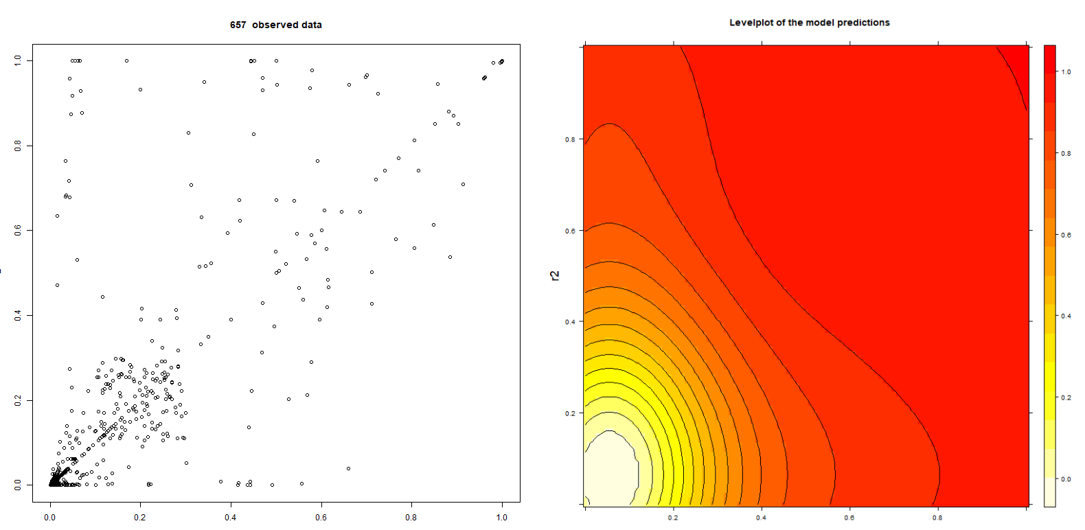
The following pictures show 657 data points of BehavioSecSession and BehavioSecTransaction plug-in risk scores (denoted by r1 and r2) from a nevisDetect test system and a level plot of the trained normalization:
Note that the data are not realistic, since the test system has frequently being used for demonstration purposes with a confidence threshold of 0.0.

The advantages of the probability density based model are:
- Training the model is fast, stable, and also suited for a large training data set.
- The Proximity property is fulfilled.
The disadvantages are:
- The assumption of statistical independence of the plug-in risk scores does not hold.
- The desired property of Monotonicityis in general not fulfilled.